Quantum vs Classic

Position 449 on the leaderboard, first try. Then we swapped the CPU for qubits. Here's what happened.

The Competition

Kaggle Playground Series S6E4 — Predicting Irrigation Need — dropped in April 2026. The task: classify agricultural fields as needing Low, Medium, or High irrigation based on soil conditions, weather, and crop type. 630,000 training rows, 270,000 test rows, 19 features, and a metric of plain accuracy — submit text labels, not probabilities.

We had a pipeline ready. The moment the competition opened, we had data downloaded, a baseline notebook running, and a submission file generated — all within the same session.

First submission: position 449 out of 768 teams. OOF accuracy 98.49%.

Not bad for a cold start. Here's how we got there, and what happened when we tried to replace the CPU with a quantum computer.

The Classical Pipeline

Data

The target distribution told us the first challenge immediately:

| Class | Count | Share | |---|---|---| | Low | 369,917 | 58.7% | | Medium | 239,074 | 38.0% | | High | 21,009 | 3.3% |

High irrigation need — the hardest class to predict — appears in only 1 in 30 rows. Miss it and you're leaving points on the table.

Feature engineering was straightforward:

Crop_Growth_Stage has a natural agronomic order (Sowing → Vegetative → Flowering → Harvest) — ordinal encoded rather than label encoded so the model can use the gradient
8 categorical columns label-encoded on the train set, applied to test
Derived features: WaterDeficit (rainfall minus soil moisture proxy), HeatStress (temperature × aridity), SunDryIndex, log transforms of skewed columns

One bug caught early: the dataset uses 'Harvest' not 'Harvesting'. The ordinal map missed it, silently producing 167,689 NaN values across the training set. Caught before submission — 0 nulls on the clean run.

The Model

Five base models trained with 5-fold stratified cross-validation, out-of-fold (OOF) predictions fed to a Logistic Regression meta-learner. The same stacking architecture that's been battle-tested across three previous competitions in this series.

base_models = [
    RandomForestClassifier(class_weight='balanced', ...),
    ExtraTreesClassifier(class_weight='balanced', ...),
    XGBClassifier(objective='multi:softprob', num_class=3, ...),
    LGBMClassifier(class_weight='balanced', objective='multiclass', ...),
    CatBoostClassifier(loss_function='MultiClass', ...),
]
meta = LogisticRegression(C=0.1)

class_weight='balanced' on the tree models was essential — without it, the 3.3% High class gets drowned out.

Result: OOF accuracy 98.49%, LB position 449.

The Quantum Experiment

With the classical submission done, we ran a parallel experiment: replace the classical models entirely with a quantum kernel SVM using IBM's Qiskit framework. Same data, same preprocessing, same evaluation. The only difference: instead of a CPU computing the decision boundary, quantum circuits on a simulated IBM QPU.

How It Works

A classical SVM with an RBF kernel computes similarity between data points using a Gaussian function. A quantum kernel SVM does the same thing, but defines similarity using quantum circuits.

The ZZFeatureMap encodes each data sample as a set of rotation angles on 4 qubits. To compare two samples, it builds a circuit called UnitaryOverlap — applying one sample's encoding circuit forward, the other's in reverse — and measures all qubits. The kernel value K(x_i, x_j) is the probability of measuring the all-zeros bitstring |0000⟩.

The feature map circuit — what runs for every data sample:

ZZFeatureMap circuit — 4 qubits, reps=2

The overlap circuit — what runs for every pair of samples to compute one kernel entry:

UnitaryOverlap circuit — U†(x_i)·U(x_j)

This is not a metaphor. It is literally:

K(x_i, x_j) = P(measure |0000⟩ after running U†(x_i) · U(x_j))

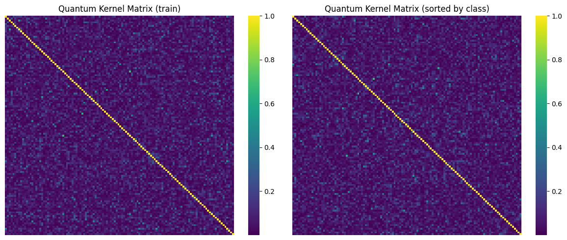
The kernel matrix itself — each cell is one quantum circuit result. Brighter = more similar samples. You want to see block structure (same-class samples clustering together):

Quantum kernel matrix heatmap

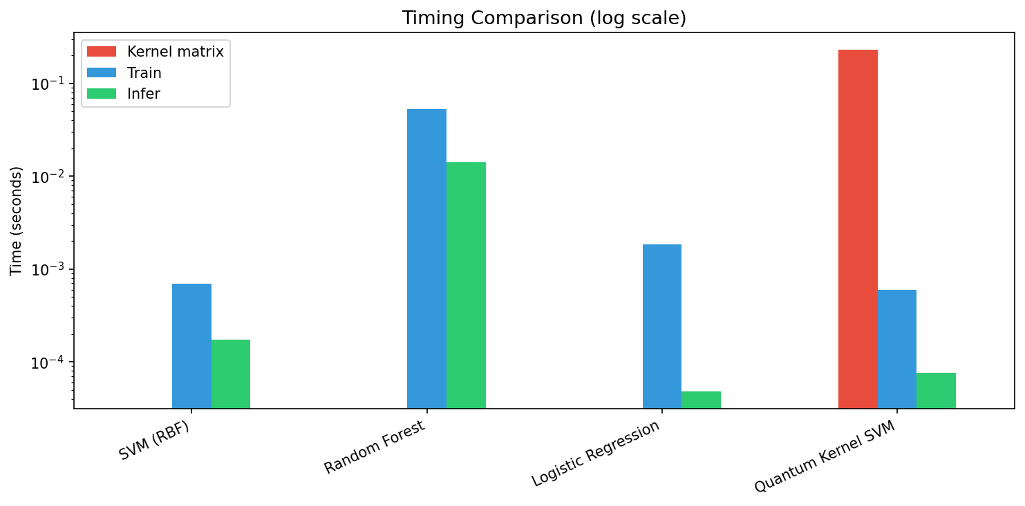
For 120 training samples, that's 7,260 unique circuit pairs. Each one a quantum computation. The full 120×120 kernel matrix was computed in 0.26 seconds using a local statevector simulator.

The Results

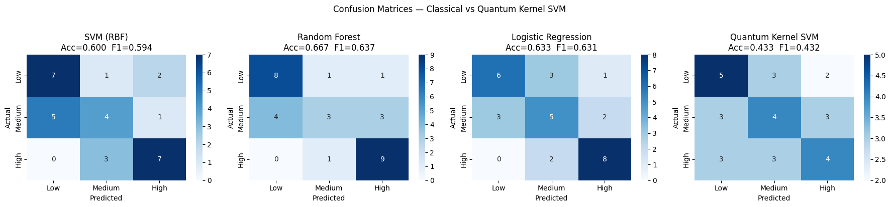
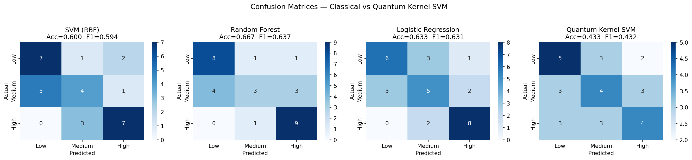
| Model | Accuracy | F1 (macro) | |---|---|---| | Random Forest | 0.667 | 0.637 | | Logistic Regression | 0.633 | 0.631 | | SVM (RBF kernel) | 0.600 | 0.594 | | Quantum Kernel SVM | 0.433 | 0.432 |

The quantum kernel SVM scored 43.3% accuracy on a 3-class problem where random chance is 33.3%. It barely beat guessing.

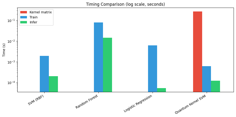
Confusion matrices for all four classifiers

The timing gap is where the engineering challenge becomes visceral:

Timing comparison — log scale

The Analogy: Echolocation in a Lit Room

Imagine you've lost your keys somewhere in your house. You have two options:

Option A: Turn on the lights and look around.

Option B: Use echolocation �� emit high-frequency pulses and analyse the interference patterns bouncing back off every surface to reconstruct the room in 3D.

Echolocation is extraordinary technology. Bats navigate pitch-black caves at speed. Submarines detect objects through miles of ocean. The technique works by exploiting wave interference — the way signals overlap and cancel and amplify depending on what they've reflected off.

But your keys are on the kitchen table. In a lit room. Echolocation doesn't help — it adds enormous complexity to a problem that has a simple, visible answer.

The quantum kernel was doing echolocation in a lit room.

Quantum kernels look for structure by measuring quantum interference patterns between data samples — the way quantum states overlap and cancel in Hilbert space. This is genuinely powerful when the data has quantum interference structure: molecular energy landscapes, quantum material phases, particle physics events. These are problems where the relevant patterns are fundamentally wave-like and exponentially complex.

Irrigation prediction is not one of those problems. The decision boundary is essentially: if the soil is dry, the temperature is high, and it hasn't rained — irrigate. That's a bright light in a lit room. Random Forest found it with axis-aligned splits in milliseconds. The quantum kernel spent 0.26 seconds computing wave interference patterns that weren't there.

The Physics: What Qubits Are Actually Good At

The confusion usually comes from conflating processing power with the right tool for the job. Quantum computers are not faster CPUs. They are not better GPUs. They are a fundamentally different computational model that is advantageous for a narrow but important class of problems.

Where quantum has genuine theoretical advantage

1. Simulation of quantum systems This is the original and strongest case — Richard Feynman's 1981 proposal that motivated the entire field. Simulating how molecules behave requires tracking quantum states that scale exponentially with classical hardware. A 50-atom molecule has 2⁵⁰ possible quantum states — classically intractable, naturally represented on 50 qubits.

Drug discovery (protein folding, binding energy prediction)
Battery materials (lithium-ion, hydrogen storage)
Fertiliser production (nitrogen fixation — the Haber-Bosch process uses 1-2% of world energy; a quantum-optimised catalyst could cut that dramatically)

2. Optimisation over exponential search spaces Quantum annealing and variational algorithms (QAOA) can explore combinatorial search spaces that are exponentially hard classically.

Logistics (vehicle routing, supply chain scheduling)
Portfolio optimisation (selecting from billions of asset combinations)
Protein structure prediction

3. Cryptography Shor's algorithm factors large integers exponentially faster than classical algorithms — breaking RSA encryption. This is why governments are investing heavily in post-quantum cryptography. It's also the most mature quantum algorithm, though the qubit counts needed are still beyond current hardware.

4. Quantum ML — but only on quantum data Quantum kernel methods are genuinely interesting when the data originates from a quantum process. If you're classifying quantum material phases from a quantum simulator, the feature map can be designed to mirror the generating process. The kernel then captures structure that no classical kernel can efficiently approximate.

For tabular Kaggle data: no.

The honest state of play

Current quantum hardware (NISQ — Noisy Intermediate-Scale Quantum) has 100–1,000 qubits, but with significant noise. Circuit depth is limited because errors accumulate with each gate. The quantum kernel experiment here used a local statevector simulator — perfect, noiseless quantum computation. On real IBM hardware, the same 4-qubit circuit would need error mitigation, and the kernel matrix would take 30–120 minutes instead of 0.26 seconds.

The gap between quantum theory and quantum practice is still large. But for quantum chemistry, materials science, and certain optimisation problems, it's closing.

What We Learned

The 98.49% OOF classical accuracy shows the problem is genuinely well-structured for tree-based models. The data is synthetic — generated from a decision-tree-like process — which is exactly why Random Forest found the boundary so cleanly.

The 43.3% quantum accuracy shows the mismatch between tool and problem. The ZZFeatureMap's inductive bias is designed for IQP-circuit-like data structure. This data doesn't have it.

The interesting finding was that PCA explained 100% of variance with just 4 components across 11 numerical features. The dataset lives in a 4-dimensional linear subspace — about as classically-tractable as data gets. Quantum advantage requires high-dimensional entangled structure. This was the opposite.

The right mental model going forward:

Use quantum when the data was born quantum. Use classical when the data was born from human decisions, sensors, and spreadsheets.

Irrigation scheduling belongs to the second category. Molecular drug binding belongs to the first. The algorithms know the difference, even if we're still learning it.

Next Steps on the Leaderboard

Position 449 is a solid baseline — top 60% on the first submission. The gap to the top is in tuning: Optuna hyperparameter search on LightGBM and XGBoost, pseudo-labelling the high-confidence test predictions, and potentially feature interactions between Irrigation_Type and soil conditions.

Takeaway

The quantum experiment runs alongside this as a research thread, not a competition strategy. When a real quantum-origin dataset turns up on Kaggle — and eventually one will — we'll be ready.